Real-time quantitative PCR (qPCR) is a powerful and commonly used method for quantifying gene expression. It is an accessible technology that can be quickly learned. However, by keeping a few key steps in mind as you plan and run your real-time PCR experiments, you can optimize your qPCR experiments and ensure high quality data and reproducible results.
Follow best practices for primer design
Primer design and validation are of primary importance in ensuring specific and efficient amplification of your target sequences. As you design your primer and amplicon sequences follow the simple primer and amplicon design guidelines outlined in Table 1. To further optimize your primer design take advantage of programs like Primer-BLAST and MFOLD. Primer-BLAST lets you design and test primers in silico to help ensure that each primer pair only amplifies your target amplicon. MFOLD can be used to screen selected amplicons for secondary structures that could prevent efficient amplification.
There are also a number of online primer databases that catalog previously designed primers. When using these primers, make sure that they perform well under your specific reaction conditions as a number of factors including your source material quantity and quality, as well as choice of polymerase or mastermix, can affect primer performance. What works in one experiment may not necessarily work in yours.
Another option is to use predesigned and wet lab validated primers. A number of manufacturers offer such primers targeting an extremely wide range of genes in multiple species. If your experiment will analyze many genes at once, predesigned primers with known reaction efficiencies can save significant amounts of time in your experimental design and testing phase.
Table 1. Primer and amplicon design guidelines
| Target Sequence/Amplicon | Primers | |
| Length, bp | 75–150 | 18–22 |
| GC content, % | 50–60 | 50–60* |
| Tm, °C | N/A | 55–65 |
| Secondary structure | Avoid | Avoid |
*Avoid long GC stretches in primers and try to design primers with a G or C at their ends
Optimize reaction conditions
If you are designing primers yourself, it is beneficial to test and optimize the annealing temperature for your primer sets (Figure 1A). Identifying and running reactions using a cycling step optimized for your primer’s annealing temperature will generate qPCR results with better reaction efficiency.
When determining the optimal annealing temperature for your primer pair, the annealing temperatures that produce the lowest Cq values will typically provide the highest sensitivity and best reaction efficiencies. An instrument with a thermal gradient function is useful at this step as it allows you to test multiple annealing temperatures in the same run. Additionally, the specificity of your reactions at different annealing temperatures can be tested with a melt step (Figure 1B). This will allow you to assess whether your primers are forming primer dimers or are amplifying non-target sequences.
Annealing temperature is especially important when performing multiplex qPCR where multiple primer pairs have to anneal at the same temperature. For these experiments it is important to determine an annealing temperature that allows efficient amplification of all amplicons. An instrument with a thermal gradient feature is particularly useful here. Alternatively, predesigned and validated primers often have annealing temperatures designed to be very similar, so using these can save time when doing multiplex qPCR.
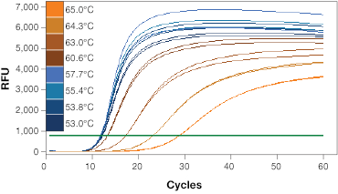
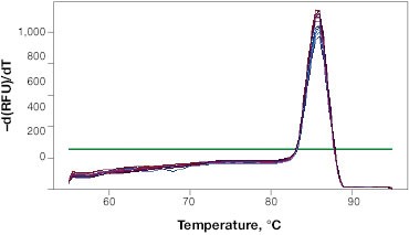
Fig. 1. Validation of qPCR primers. A, qPCR is performed at a range of annealing temperatures using a thermal gradient block. Amplification profiles indicate that the most efficient amplification occurs at the four lowest annealing temperatures between 53 and 57.7°C where the curves are at the lowest Cq. B, a single peak on the melt curve analysis indicates a single PCR product. RFU, relative fluorescence units.
Coming Soon
Bio-Rad is launching a new qPCR analysis software, with even more features to support easy production of reliable and reproducible qPCR data. Sign up to be notified when the software launches.
Keep Me InformedAssess reaction efficiency
Knowing the specific amplification efficiency for your qPCR primers and reaction conditions lets you ensure that your reactions are running well. Additionally, if performing relative normalized expression analysis, incorporating known reaction efficiencies into Cq calculations will produce more accurate values.
To determine reaction efficiencies, generate a standard curve from a serial dilution of template containing your target gene and perform a qPCR run on this dilution series. Ideally, a standard curve will cover a large concentration range – a series of 8 dilutions at 10x will provide a broad range for analysis. Efficiency is calculated by analyzing the Cq values for all points of the standard series. A primer pair should amplify a target sequence with a reaction efficiency between 90% and 110%. Good qPCR software should have a function that automatically calculates reaction efficiencies, simplifying this step. Additionally, good software can automatically use these efficiencies in your experiments when calculating relative normalized gene expression levels.
Pick a stable reference gene
When comparing qPCR results from different source material, a reference gene that is expressed at the same level in all samples serves as a way to normalize for different overall starting levels of RNA or slight sample to sample differences in reaction efficiency. Often researchers will pick a common reference gene, such as GAPDH or ACTB, and assume that this gene is stable (expressed at the same level in all of their samples and under all experimental conditions). However, several studies suggest that expression of these genes can vary significantly in different systems. You can therefore further improve data quality by testing potential reference genes for stability.
The geNorm method (Hellemans et al. 2007) provides a way to analyze the stability of potential reference genes. To use the geNorm method, first run a qPCR reaction and determine expression levels of your potential reference genes. Then apply the geNorm algorithm to your results. The geNorm algorithm when applied, produces an M value for each potential reference gene. A good reference gene will have an M value below 0.5 in homogeneous and 1 in heterogeneous samples sets (Vandesompele et al. 2002). To make this process even easier, some qPCR software packages will automatically run geNorm analysis and identify ideal reference genes for your experiment (Figure 2).
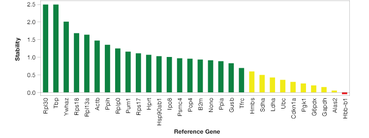
Fig. 2. Reference gene stability can vary greatly. The most stable genes for this experiment are shown in green, depicted as Ln(1/M) where M is the value produced using the GeNorm algorithm.
Design for consistency and experimental reproducibility
As with any scientific experiment or study, conscientious experimental design is important in qPCR. There can be many potential sources of variability in real-time PCR experiments; two common ones that we can attempt to control for are biological variability and technical variability in the qPCR process. Biological variability is due to inherent differences between individual organisms, tissues or cell culture samples. Technical variability is introduced during the experiment through factors such as variability in the total volume of liquid pipetted or in sampling variability.
To account for technical variability, include at least two technical replicates for every sample and experimental condition. Technical replicates are reactions that we expect to have identical contents; any measured differences can be attributed to technical (or experimental) variability. To account for biological variability it is best to include at least three biological replicates per sample and condition. These should be samples taken from the same tissue of one organism, or may also be samples from multiple organisms, grouped together for analysis (for example, multiple mice from the same treatment group may be considered and analyzed together in the same biological group) (Figure 3).
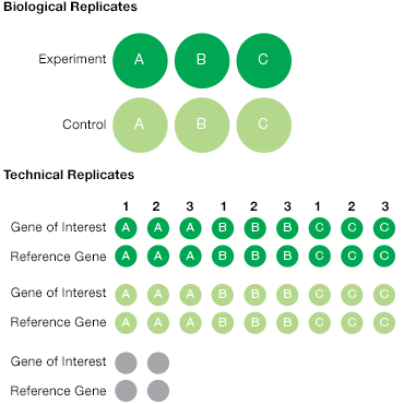
Fig. 3. Experimental replicates. All experiments should be designed with a combination of biological and technical replicates. This illustrates a simple experiment with triplicate biological samples from control (![]() ) and treatment experimental (
) and treatment experimental (![]() ) conditions. For each biological sample, three technical replicates are recommended for the gene of interest as well as for the reference gene(s). This results in a total of at least 36 samples plus the duplicate NTC (
) conditions. For each biological sample, three technical replicates are recommended for the gene of interest as well as for the reference gene(s). This results in a total of at least 36 samples plus the duplicate NTC (![]() ) for a total of >40 wells.
) for a total of >40 wells.
If performing a multi-plate study, you can save yourself time and headache by utilizing a common nomenclature across all plates in the study. This is especially important if you have samples that are part of the same biological group but run on different plates. If naming conventions are not consistent, your data may not be grouped or analyzed correctly. Additionally, it is ideal to run a common sample with a known quantity of DNA on each plate. This sample can be used as a calibrator to normalize the results of each plate and account for any run-to-run variability.
Once you have determined your samples, replicates, and any controls, don’t forget to design and lay out your plate and samples correctly in your qPCR analysis program. This helps to ensure that all calculations and analyses are done correctly, on the right samples. This is again an area where well-designed qPCR software that allows for the designation of both technical and biological replicates during plate setup can help. You can then group these replicates together for analysis, so that the effects of both process variability and biological variability can be easily viewed, accounted for, and taken into consideration in calculations.
Ensure statistical significance of your results
Once you have designed, validated, and run your experiment you likely will need to determine whether differences between biological groups or samples are statistically significant or whether they can be explained by the variability in a single population. This can be accomplished using a t-test, ANOVA, or other statistical technique. Programs like GraphPad or qPCR-specific software such as qbase+ can be used to perform statistics on your results. Some qPCR instrument software programs also include statistical analysis features, allowing you to rapidly collect and analyze your data in a single program.
Following these key steps in designing and performing real-time PCR experiments will help you to produce high quality and reproducible data. For a more detailed discussion, download our Practical Approach to RT-qPCR.
References
Hellemans J et al. (2007). qbase relative quantification framework and software for management and automated analysis of real-time quantitative PCR data. Genome Biol 8, R19.
Vandesompele J et al. (2002). Accurate normalization of real-time quantitative RT-PCR data by geometric averaging of multiple internal control genes. Genome Biol 3, research 0034.1–0034.11.