End the Cycle of Repeated, Failed Experiments with a Robust Field Guide to qPCR

Introduction

qPCR has become a ubiquitous technology for nucleic acid detection and quantification. It remains the gold standard for validation of microarray and next generation sequencing data and the method of choice for both clinical and basic research labs for a wide range of applications that include: 1) monitoring viral and bacterial infection; 2) tracking environmental microbial populations; and 3) the quantification of differential gene expression levels between experimental groups. However, there remains general concern about the production of data that truly reflects the tested experimental conditions (Bustin and Nolan 2017). This stems from the general perception that the generation of qPCR amplification curves and Cq values implies the production of interpretable data. Unfortunately, qPCR itself is highly robust and can yield Cq values regardless of the level of sample quality and purity. Only data generated from samples and primers that have undergone rigorous validation will ensure accurate and reproducible interpretations.

Producing Publication-Quality, Reproducible Data the First Time:

2019’s best review in Trends in Biotechnology.

Without following a rigorous, stepwise approach and checkpoints throughout a given qPCR experiment, the results and conclusions can be far from valid or reproducible. This has led to a growing number of questionable articles employing qPCR, estimated to total well above 50% of the published literature (Bustin and Nolan 2017). To assist the scientific community in publishing high-quality, reproducible data that reflect true experimental conditions, we have developed a comprehensive guide to performing the ultimate qPCR experiment. The following is a snapshot of the critical steps needed to achieve excellent results.

A guided, rigorous approach to qPCR

Step 1 — Experimental Design

Take the time to design the experiment bearing in mind that qPCR is one of the most sensitive molecular biology assays (Figure 1A). The advantage of sensitivity is the detection and quantification of low-abundance targets, which are often the most interesting. However, the disadvantage is the high potential for producing artefactual data from a poorly designed experiment. The assessment of time points (Figure 1B) and tissue sub sections (Figure 1C) coupled with the selection of an appropriate number of biological replicates per treatment group are good examples of key design parameters that are essential considerations to assure publication of precise, accurate, and reproducible data.

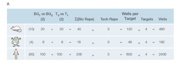
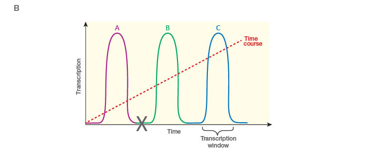
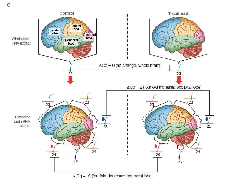
Fig. 1. Planning and scoping a quantitative PCR (qPCR) experiment. A, biological group (BG): tested experimental conditions (i.e., control (BG1) vs treatment (BG2). Time point (T) (i.e., 0 hour (T0) and 1 hour (T1) post-treatment). Biological replicate (Bio reps): number of independent biological specimens from which cDNA/gDNA is produced (i.e., individual samples). Technical replicate (Tech reps): number of repeats per Bio rep (i.e., same cDNA/gDNA sample pipetted into multiple wells). Targets: genes interrogated for differential expression or abundance including chosen reference genes. Wells: total number of microtiter plate wells required for qPCR exclusive of optimization experiments for primer validation (see Figure 2). B, time dependence on transcription of targets A, B, and C post-treatment. Choosing a random time point (X) post-treatment may result in no data and/or artefactual data that do not reflect the true response of the tested targets. Performing a preliminary time course study (dotted line) ensures the selection of optimal time points for each target. C, influence of tissue sectioning on data quality. Whole tissue RNA extract may show no change, whereas dissected tissue may produce expression differences between biological groups (i.e., fourfold change when comparing expression of occipital lobe or temporal lobe) consequent to target dilution in whole tissue and enrichment in sections. Adapted and updated under a Creative Commons license from Taylor et al. 2019.

Step 2 — Sample Extraction and Nucleic Acid Isolation

Harvest the samples with appropriate kits, reagents, and instrumentation to minimize time and maximize yield in isolating RNA or DNA. A good nucleic acid purification methodology will reduce protein and chemical contaminants that can partially inhibit the reverse transcription and qPCR reactions or perturb primer annealing (Gibson et al. 2012, Tan and Yiap 2009). This can dramatically alter the Cq values producing data and interpretations that are unrelated to the tested experimental conditions. A good kit, such as the Aurum Total RNA Isolation Kits from Bio‑Rad, assures high-quality samples with excellent purity. RNA and DNA samples should be assessed for purity using a spectrophotometric method and for quality by either running a gel or using a Bioanalyzer System.

Step 3 — Reverse Transcription

For RNA isolation, use a good reverse transcription (RT) kit to produce a complete and representative cDNA copy of the mRNA. The hallmarks of a good RT kit include: 1) a mixture of random hexamers and oligo(dT)s to assure complete coverage of the transcriptome; 2) RNase H to digest the RNA while the cDNA is synthesized, which minimizes bias in cDNA production preventing the Cq values from being skewed to lower and variable values that would be unrepresentative of the true target amount in each sample; 3) an RNase inhibitor to prevent degradation of the RNA prior to RT; 4) a highly robust RT enzyme that permits RT of the widely ranging concentration of transcripts populating each sample. iScript Reverse Transcription Reagents from Bio‑Rad contain a blended mixture of each of these components to assure cDNA that closely reflects the transcriptome.

Step 4 — Primer Validation

Validate primers initially with a thermal gradient to assess annealing temperature followed by a standard curve to assess reaction efficiency (Figure 2A). Use an equalized pool of cDNA from all of the experimental groups including control for both primer validation experiments. Thermal validation assures that primer annealing is optimized based on the unique salt concentration, pH, and contaminants in the experimental samples (Figure 2B). The standard curve permits a guided approach to correctly diluting individual samples to ensure adequate contaminant and transcript dilution such that the reaction efficiency for each primer pair is close to 100% (Figure 2C). Only under these conditions will the Cq values reflect the true target concentrations for accurate interpretations. A good qPCR supermix can help assure solid results; the SsoAdvanced Universal Inhibitor-Tolerant SYBR^® Green Supermix from Bio‑Rad contains a chimerized Taq polymerase that is more inhibitor tolerant to give better reproducibility between individual samples with variable levels of contaminants.

Step 5 — Reference Gene Selection

Test a panel of at least seven to ten reference genes to uncover two or three that are stably expressed between the treatment groups. Poor reference gene selection can dramatically alter the data and produce misleading conclusions (Figure 2D) (Robledo et al. 2014, Vandesompele et al. 2002). PrimePCR Assays are wet-lab validated and sequence-verified primers from Bio‑Rad for several genomes, including human, mouse, and rat. These assays can be purchased individually or in panel assays with suggested reference gene targets that can be assessed for stability between the experimental groups.

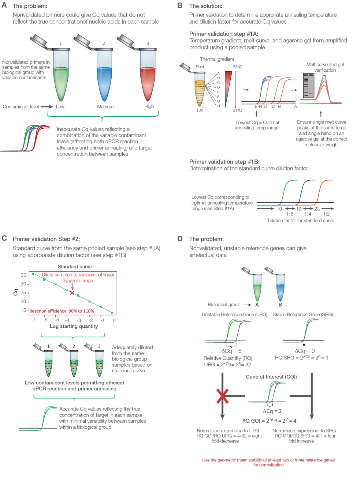
Fig. 2. Validating a quantitative PCR (qPCR) experiment to minimize error and maximize data quality. A, nonvalidated primers could give variable and/or artefactual data that do not reflect the true target abundance in each sample. B, primer validation using thermal gradient and gel electrophoresis. Step #1A: Thermal gradient and agarose gel validation. To validate primers, an equalized pool of samples from each biological group is diluted 1:20 and initially tested using a thermal gradient to determine the optimal annealing temperature, average level of expression, and unique product for each target from melt curve and gel analysis. Step #1B: The quantitative cycle (Cq) value from the optimal annealing temperature range can be used as a guide to establish the standard curve dilution factor for each target (i.e., if the Cq value for optimized temperature range is between 10 and 16, use a 1:8 serial dilution series of the pooled cDNA sample in water). C, standard curve validation. An eight-point standard curve is tested for each primer pair using the same pooled sample and the appropriate dilution factor as determined from the thermal gradient data (Step #1B) to cover the widest dynamic range possible. Amplification efficiency, as determined from the slope, should range between 90% and 110%. Deleting the highest and/or lowest concentration points from each primer validation standard curve may be necessary to achieve the best efficiency. The dilution factor from the midpoint is then used to dilute the individual experimental samples per target, assuming that the pooled DNA sample represents the average abundance of each target for the experiment (i.e., equalized pool of the same number of DNA samples from each biological group). This ensures minimal presence of contaminants affecting primer efficiency and accurate quantitative data. D, consequence of using poorly validated reference genes. qPCR data can change dramatically when normalization is performed using a stable versus unstable reference gene. Adapted and updated under a Creative Commons license from Taylor et al. 2019.

Step 6 — Working Up the Data

Apply care in performing the calculations for relative gene expression (Figure 3). There are several steps and multiple formulas required for qPCR data analysis and many labs employ Excel spreadsheets. Since qPCR experiments often require combining data from multiple plates, copy/paste and formula propagation errors can yield inaccurate data and interpretations that are very challenging to recognize and troubleshoot. CFX Maestro Software is a solution from Bio‑Rad that is paired with data generated from our qPCR instruments, permitting the data produced from a given project to be calculated seamlessly, reproducibly, and correctly for multiple plates. Since the raw data never leaves the software and the calculations are based on both the Pfaffl (Pfaffl 2001) and Vandesompele (Vandesompele et al. 2002) methods, the risk of data-manipulation errors is eliminated and ensures that all lab members are producing consistently and correctly calculated final results.

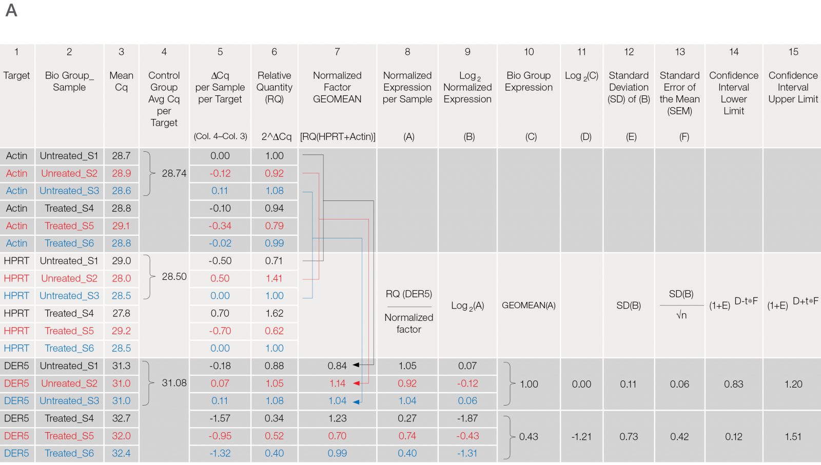
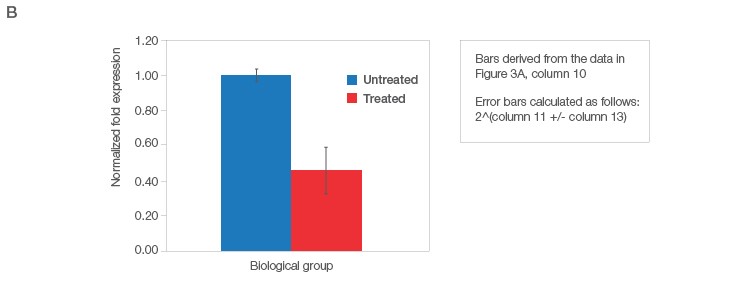
Fig. 3. Data analysis for a typical relative quantification experiment. A, rigorous data workup. In this example, DER5 expression is measured between treated and untreated biological groups, each containing three biological replicates and two technical replicates (data for technical replicates is not shown). Actin and HPRT are used as reference genes. First, the mean quantitative cycle (mean Cq; column 3) of the technical replicates for each sample/target combination is calculated [i.e., for actin from the untreated sample 1 (Untreated_S1) the mean Cq is 28.7]. The average Cq of all samples in the control group (i.e., untreated) for each target is then determined (column 4). The relative difference (ΔCq) between the average Cq for the control group (column 4) and the mean Cq (column 3) per individual sample within each target is assessed (column 5). The relative quantities are calculated from the ΔCq (i.e., 2ΔCq) where in this case, it is assumed that reaction efficiency is 100%, and hence a base of two is applied (column 6). Otherwise the base should be one + PCR efficiency (E) [as determined from the standard curve (Figure 2C)]. In effect, the relative quantity represents the fold change between the biological groups for each sample/target combination prior to reference gene normalization. For each biological group/sample combination, a normalization factor is determined from the geometric mean of the associated reference gene relative quantities (column 7). The relative normalized expression for each target gene (DER5 in this example) is then calculated per sample by dividing the relative quantity by the normalization factor (column 8) followed by log transformation (column 9). The average relative normalized and log transformed expression for each biological group is then calculated using the geometric mean (columns 10 and 11). The standard deviation (SD), standard error of the mean (SEM), and 95% confidence interval [in this case a t statistic of 4.3 was used based on three samples per biological group (i.e., 2 degrees of freedom)] of each group are then calculated from the log transformed normalized expression (columns 12–15). B, average relative normalized expression graphical representation with appropriate error bars (in this case SEM). Adapted and updated under a Creative Commons license from Taylor et al. 2019.

Conclusions

Although it is easy to produce data from qPCR reactions, only through the application of a rigorous, stepwise approach will the data and interpretations be reflective of the tested experimental conditions. Bio‑Rad not only offers excellent reagent and instrument solutions but also a superior technical team to guide and support the scientific community in producing excellent results.

To learn the fundamentals and best practices of qPCR and to schedule a departmental qPCR workshop with a member of our Field Application Scientist team, contact your local Bio‑Rad representative today.

Open access article: Trends in Biotechnology, July 2019, Vol. 37, Issue 7, P761-774.

YouTube Tutorial Video Series Playlist “Achieving the Ultimate qPCR Experiment Tutorial Videos”.

References

SYBR is a trademark of Thermo Fisher Scientific Inc. Bio‑Rad Laboratories, Inc. is licensed by Thermo Fisher Scientific Inc to sell reagents containing SYBR Green I for use in real-time PCR, for research purposes only.

References

Bustin S and Nolan T (2017). Talking the talk, but not walking the walk: RT-qPCR as a paradigm for the lack of reproducibility in molecular research. Eur J Clin Invest 47, 756–774.
Gibson KE et al. (2012). Measuring and mitigating inhibition during quantitative real time PCR analysis of viral nucleic acid extracts from large-volume environmental water samples. Water Res 46, 4,281–4,291.
Pfaffl MW (2001). A new mathematical model for relative quantification in real-time RT-PCR. Nucleic Acids Res 29, e45.
Robledo D et al. (2014). Analysis of qPCR reference gene stability determination methods and a practical approach for efficiency calculation on a turbot (Scophthalmus maximus) gonad dataset. BMC genomics 15, 648.
Tan SC and Yiap BC (2009). DNA, RNA, and protein extraction: the past and the present. J Biomed Biotechnol 2009, 574398.
Vandesompele J et al. (2002). Accurate normalization of real-time quantitative RT-PCR data by geometric averaging of multiple internal control genes. Genome Biol 3, RESEARCH0034.
Taylor SC et al. (2019).The ultimate qPCR experiment: Producing publication quality, reproducible data the first time. Trends Biotechnol [published online ahead of print January 14, 2019]. Accessed May 29, 2019.